Diffraction Integral
In the last section about Fresnel zones and the zone plate, we considered how different paths contribute to the intensity at a point on the optical axis. We would like to generalize this idea to an integral formulation that allows us to calculate any kind of diffraction pattern.

Assume we have a light source \(S\) as shown in the image above, which emits a spherical wave (though it does not necessarily have to be a spherical wave). The spatial amplitude of this wave at the point \(P(x,y)\) at a tiny aperture element \(d\sigma\) is given by:
\[ U_s(x,y) = U_0(x,y)e^{i\phi(x,y)} \]
where
\[ U_0 = \frac{A}{R} = \frac{A}{\sqrt{g^2 + x^2 + y^2}} \]
and
\[ \phi(x,y) = -kR \]
This represents the amplitude of the Huygens wave, which emanates from the point \(P(x,y)\) and propagates towards the screen at \(P(x',y')\). This Huygens wave contributes a fraction of an amplitude \(dU_p\) to the total amplitude at point \(P(x',y')\), which is given by:
\[ dU_p = C \frac{U_s d\sigma}{r} e^{-ikr} \]
with \(C = \frac{i \cos(\theta)}{\lambda}\), known as the obliquity factor, found through a more detailed calculation.
The total amplitude at the point \(P(x',y')\) is then given by the integral over all contributions:
\[ U_p = \iint C U_s \frac{e^{-ikr}}{r} dx dy \]
where \(dx dy = d\sigma\). The integral runs over all positions in the aperture plane \((x,y)\) where there is an opening. This integral is called the Fresnel-Kirchhoff diffraction integral and allows us to calculate complex scalar diffraction patterns.
This formulation generalizes the concept of Fresnel zones and provides a powerful tool for analyzing and predicting diffraction patterns for various aperture shapes and configurations.
Fresnel Approximation
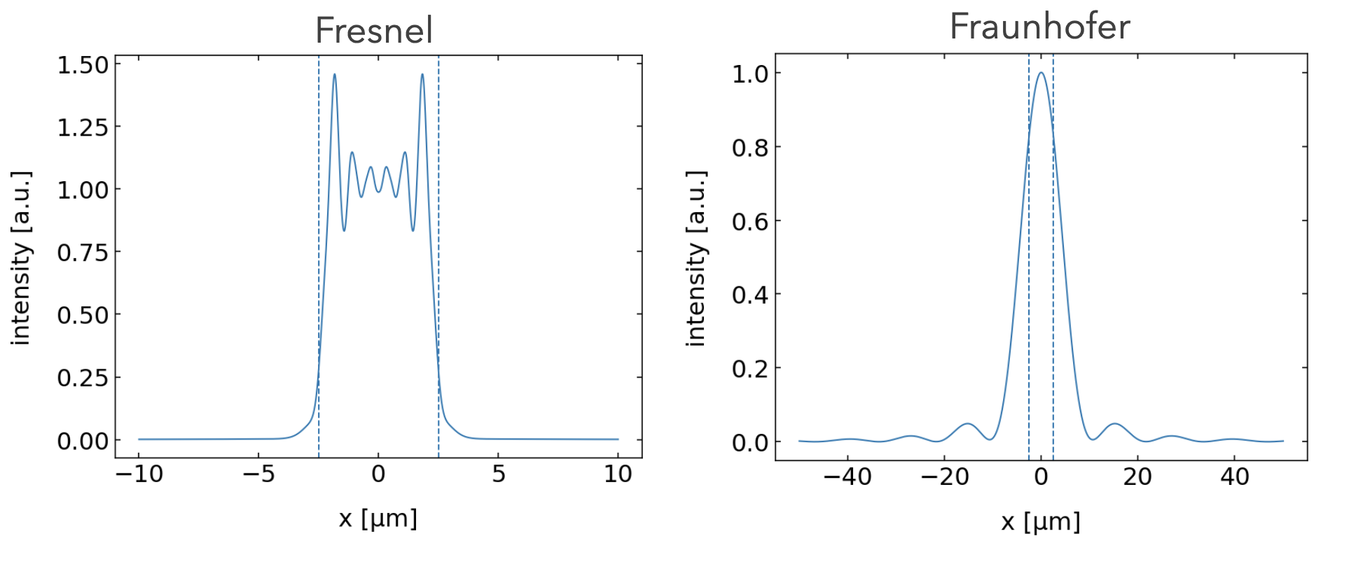
The diffraction integral does not always need to be calculated in full; we can use approximations to obtain diffraction patterns in different regimes. One such approximation is the Fresnel approximation, which yields the diffraction pattern in the near field.
The distance \(r\) from the point \(P(x,y)\) to the point \(P(x',y')\) can be written as:
\[ r = \sqrt{z_0^2 + (x - x')^2 + (y - y')^2} \]
Using a binomial expansion for small angles, we can approximate this as:
\[ r \approx z_0 \left(1 + \frac{(x - x')^2}{2z_0^2} + \frac{(y - y')^2}{2z_0^2} + \ldots \right) \]
In this approximation, we assume that \(\cos(\theta) = z_0 / r \approx 1\) and \(C = i / \lambda\), considering small diffraction angles. Using this approximation, we find the amplitude of the wave at a point \(P(x',y')\):
\[ U(x', y', z_0) = i \frac{e^{-ikz_0}}{\lambda z_0} \iint U_s(x, y) \exp \left[ -\frac{ik}{2z_0} \left( (x - x')^2 + (y - y')^2 \right) \right] dx dy \]
As the integration is over \(x\) and \(y\), we can factor out all screen coordinate elements, yielding:
\[ U(x', y', z_0) = i \frac{e^{-ikz_0}}{\lambda z_0} e^{-\frac{ik}{2z_0}(x'^2 + y'^2)} \iint U_s(x, y) e^{-\frac{ik}{2z_0}(x^2 + y^2)} e^{\frac{ik}{z_0}(xx' + yy')} dx dy \]
This is the Fresnel approximation. It simplifies the calculation of the diffraction pattern in the near field by making reasonable assumptions about the geometry and angles involved.
Fraunhofer Approximation
If we further assume that the aperture is small as compared to the distance at which we observe the diffraction pattern, we can further simplify the Fresnel approximation to yield the Fraunhofer approximation giving the diffraction pattern in the far field. The condition is
\[ z_0\gg\frac{1}{\lambda}(x^2+y^2) \]
In this case we can neglect the term
\[ e^{ -\frac{ik}{2z_0}(x^2+y^2)} \approx 1 \]
which results in
\[ U(x^{\prime},y^{\prime},z_0)=i\frac{e^{-ikz_0}}{\lambda z_0} e^{-\frac{ik}{2z_0}(x^{\prime 2}+y^{\prime 2})} \iint U_{s}(x,y) e^{\frac{ik}{z_0}(xx^{\prime}+yy^{\prime})} dx dy \]
The Fraunhofer diffraction formula reveals a profound relationship: the far-field diffraction pattern is the 2D Fourier transform of the aperture function. To see this, define spatial frequencies \(f_x = x'/({\lambda z_0})\) and \(f_y = y'/({\lambda z_0})\). The integral then becomes:
\[ \iint U_{s}(x,y) e^{2\pi i(f_x x + f_y y)} dx dy \]
This is precisely the Fourier transform of \(U_s(x,y)\). This connection is the foundation of Fourier optics, a powerful framework where lenses perform Fourier transforms, optical systems act as filters in frequency space, and diffraction patterns can be understood as spatial frequency spectra. This perspective enables techniques like optical image processing, holography, and the analysis of optical transfer functions.
While these formulas provide the mathematical tools, we may obtain a more intuitive idea about the different approximation in the following way. Consider the image below, where we would like to know about the diffraction intensity of a slit of width \(b\) at the optical axis at a distance \(D\).

The waves from the center of the slit and the edge have to travel towards that point a different path length, which we may calculate to
\[\begin{eqnarray} \Delta s &=& \sqrt{\frac{b^2}{4}+D^2}-D\\ &=& D\sqrt{\frac{b^2}{4D^2}+1}-D \end{eqnarray}\]
We may develop the square root into a Taylor series and obtain
\[\begin{eqnarray} \Delta s &=& \frac{b^2}{8D}-\frac{b^4}{128 D^3}+O(4)\\ &\approx & \frac{b^2}{8D} \end{eqnarray}\]
The first-order term \(\frac{b^2}{8D}\) decreases quadratically with the distance \(D\) of the point, which means that at large distances, we can safely assume \(\Delta s=0\) on the axis, i.e. all waves arriving at that point have to travel the same distance. This corresponds to the far-field approximation. To be more specific we require
\[ \frac{b^2}{8D}<\frac{\lambda}{8} \]
or
\[ \frac{b^2}{\lambda D}<1 \]
to be fulfilled to be in the far field.
\[ F=\frac{b^2}{\lambda D} \begin{cases} \ll 1 ,&\textrm{Fraunhofer}\\ \approx 1,& \textrm{Fresnel}\\ \gg 1, & \textrm{Full vector} \end{cases} \]
This number \(F\) is called the Fresnel number and gives us an idea by how far the dimensions of the opening contribute to the diffraction pattern rather than the direction of the wave propagation only.
The choice of \(\lambda/8\) in the far-field criterion is not arbitrary. A path difference of \(\lambda/8\) corresponds to a phase error of \(\pi/4\) radians (45°). This is based on the Rayleigh quarter-wave criterion, which states that phase errors below \(\pi/4\) introduce negligible wavefront distortion (less than ~8% intensity error). This threshold provides a good balance between accuracy and practical applicability in diffraction calculations. Depending on the required precision, stricter criteria (e.g., \(\lambda/16\)) or more relaxed ones (e.g., \(\lambda/4\)) may be used.
Babinet’s Principle
The above considerations of diffraction have some intriguing consequence. Consider the two apertures in the image below.

The left aperture will create in the far field an amplitude distribution \(U_h\), while the inverse aperture on the right will cause an amplitude \(U_d\). If we combine both amplitudes in the far field, we obtain a total amplitude distribution
\[ U=U_h+U_d \]
In the case when we have two complementary apertures (i.e., one is transparent where the other is opaque and vice versa), the total amplitude has to equal the unobstructed wave amplitude \(U_0\). When we consider points far from the optical axis in the far field, the unobstructed wave contribution is negligible, so we obtain
\[ U_h+U_d \approx 0 \]
and therefore
\[ U_h \approx -U_d \]
Since the intensity is proportional to the square of the amplitude magnitude, we find
\[ I_h=|U_h|^2=|U_d|^2=I_d \]
Note that this equality holds everywhere except at the forward direction (optical axis), where the unobstructed wave contributes significantly. This is the Principle of Babinet which states:
Babinet’s principle states that the far-field diffraction intensity distribution of complementary apertures is identical. This means that an opaque object and its complementary aperture (where the object is replaced by a transparent region and vice versa) produce the same diffraction pattern in the far field.
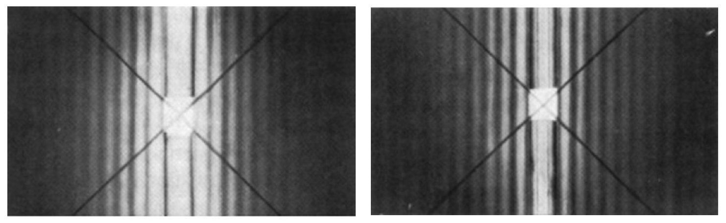
The images below show an experimental demonstration of Babinet’s principle on a slit and a wire.